A note on the complexity of the Lanczos method

Classical bounds and probabilistic estimates for eigenvalue computation

Overview

We review the standard results of Lanczos on finding eigenpairs. The Lanczos method computes the eigenvalue of symmetric matrix $A \in \mathcal{S}^n$. Assume that the eigenvalues are ordered as

$$\lambda_1 \ge \lambda_2 \ge \ldots \ge \lambda_n.$$

Without loss of generality we assume $\lambda_1 > \lambda_2$; otherwise, simply take the next eigenvalue knowing degeneracy exists.

Standard relative error to spread

For example, consider the maximum eigenvalue, the standard theory for $i$-th eigenvalue evaluates the arithmetic operations needed for an approximate eigenvalue $\xi$ to satisfy the relative error to spread,

$$0 \leq \lambda_1-\xi \leq\left(\lambda_1-\lambda_n\right) \varepsilon,$$

where $\varepsilon > 0$ is the relative error, and $\xi$, the so-called Ritz value, is taken from some iteration $k$.

Kuczyński’s relative error

Kuczyński ¹ on the other hand used a different aspect,

$$\left|\frac{\xi(A)-\lambda_1(A)}{\lambda_1(A)}\right| \leq \varepsilon,$$

One can connect this to the relative error to spread by the following inequality,

$$\frac{\lambda_1(A) - \xi(A)}{\lambda_1(A) - \lambda_n(A)} = \frac{\lambda_1(A) - \xi(A)}{\lambda_1(A - \lambda_n(A)\cdot \mathbf{I})} = \frac{\lambda_1(A - \lambda_n(A) \mathbf{I}) - \xi(A - \lambda_n(A) \mathbf{I})}{\lambda_1(A - \lambda_n(A) \mathbf{I})}.$$

This implies the relative error to spread is equivalent to the $\lambda_1(A - \lambda_n(A) \mathbf{I})$ in Kuczyński’s estimate. Since the Lanczos method is scale-invariant, the results are exactly identical.

Smallest eigenvalue

We introduce the estimate for smallest eigenvalue. This is equivalent to the largest eigenvalue of $-A$. Indeed, $\lambda_n(A) = - \lambda_1( - A)$. Suppose $-\xi$ approximates $\lambda_1( - A)$, we know by the relative error to spread the error concerns

$$\lambda_1(-A) - (-\xi) \leq\left(\lambda_1(-A) - \lambda_n(-A)\right) \varepsilon$$

One also note the original theory considers $A \succeq 0$ while $-A$ obviously does not hold. Again we use the scaling for some $M \ge \lambda_1(A)$ and the above inequality is equivalent to

$$\lambda_1(M\cdot \mathbf{I} -A) - (M\cdot \mathbf{I}-\xi) \leq\left(\lambda_1(M\cdot \mathbf{I}-A) - \lambda_n(M\cdot \mathbf{I}-A)\right) \varepsilon$$

which is equivalent to

$$\xi - \lambda_n(A) \leq \left(\lambda_1(A) - \lambda_n(A)\right) \varepsilon.$$

since the spread of $A$ is the same as $-A$ (or $M\cdot \mathbf{I} - A$)

Regarding $|A|$

Sometimes the matrix $A$ is indefinite from a Hessian matrix where Lipschitz continuity is present. For that, we usually allow for $|A|$, the induced $\ell_2$ norm. We first note all the above results are scale-invariant so the same bounds hold; granted, one can consider $A - \lambda_1(A) \mathbf{I}$ and use the smallest eigenvalue estimate. On the other hand, we can replace $\lambda_1(A) - \lambda_n(A)$ by $|A|$:

$$\|A\| = \sup _{\|x\|=1} \|A x\|= \max\{|\lambda_1(A)|, |\lambda_n(A)|\}.$$

So that

$$\lambda_1(A) - \lambda_n(A) \le 2 \max\{|\lambda_1(A)|, |\lambda_n(A)|\} \le 2\|A\|.$$

and thus the error estimates

$$\frac{\xi - \lambda_n(A)}{2\|A\|} \le \frac{\xi - \lambda_n(A)}{\lambda_1(A) - \lambda_n(A)} \leq \varepsilon$$

as it is safe to say,

$$\xi - \lambda_n(A) \leq 2 \varepsilon \|A\|.$$

Absolute error

All of above results considers relative error. For absolute error, e.g.,

$$|\lambda_1 - \xi| \le \epsilon$$

it is equivalent to say

$$\varepsilon = \frac{\epsilon}{\lambda_1(A) - \lambda_n(A)}.$$

Classical Bounds from Kaniel–Paige

Classic bounds used distribution-dependent bounds, that is, the spectrum of eigenvalues. The following theorem can be found in standard eigenvalue textbooks ².

$C(\cdot)$ is the Chebyshev polynomial of the first kind.

Chebyshev polynomial of the first kind

The $k$-th order Chebyshev polynomial of the first kind is defined as

$$C_k(t)=\cos \left[k \cos ^{-1}(t)\right], \forall t, -1 \leq t \leq 1.$$

so that,

$$C_{k+1}(t)=2 t\cdot C_k(t)-C_{k-1}(t).$$

To extend the definition to cases where $|t|>1$, we use the following formula,

$$C_k(t)=\cosh \left[k \cosh ^{-1}(t)\right], \quad|t| \geq 1.$$

This is readily seen by passing to complex variables and using the definition $\cos \theta=\left(e^{i \theta}+e^{-i \theta}\right) / 2$. As a result of we can derive the expression,

$$C_k(t)=\frac{1}{2}\left[\left(t+\sqrt{t^2-1}\right)^k+\left(t+\sqrt{t^2-1}\right)^{-k}\right]$$

and for that we know,

$$C_k(t) \ge \frac{1}{2}\left(t+\sqrt{t^2-1}\right)^k := \underline{C}_k(t), \quad \forall|t| \geq 1.$$

Largest Eigenvalue

When specifying to extreme ones ($i\in{1, n}$), we have the following corollary.

Note that $1+2\gamma_i \ge 1$ holds $\forall i \ge 1$. We are ready for the next theory,

Proof sketch: We need $k$ such that

$$\left(\frac{\tan \angle\left(b, v_1\right)}{ C_{k-1}\left(1+2 \gamma_1\right)}\right)^2 \le \varepsilon.$$

Observe if

$$\varepsilon^{-1/2}|\tan \angle\left(b, v_1\right)| \le \frac{1}{2}\left(t+\sqrt{t^2-1}\right)^k,$$

then

$$\varepsilon^{-1/2}|\tan \angle\left(b, v_1\right)| \le \frac{1}{2}\left(t+\sqrt{t^2-1}\right)^k \leq \underline{C}_{k-1}\left(1+2 \gamma_1\right) \leq C_{k-1}\left(1+2 \gamma_1\right)$$

and further

$$\frac{\tan \angle\left(b, v_1\right)}{C_{k-1}\left(1+2 \gamma_1\right)} \le \sqrt{\varepsilon}$$

as desired.

We focus on

$$\left(t+\sqrt{t^2-1}\right)^{k-1} \ge 2\cdot |\tan \angle\left(b, v_1\right)|/\sqrt{\varepsilon}, \quad \text{for some}~ t = 1+2\gamma_1$$

$$\Rightarrow k \ge 1+\log \left( \frac{2|\tan \angle\left(b, v_1\right)|}{\sqrt{\varepsilon}}\right) / \log \left(t+\sqrt{t^2-1}\right).$$

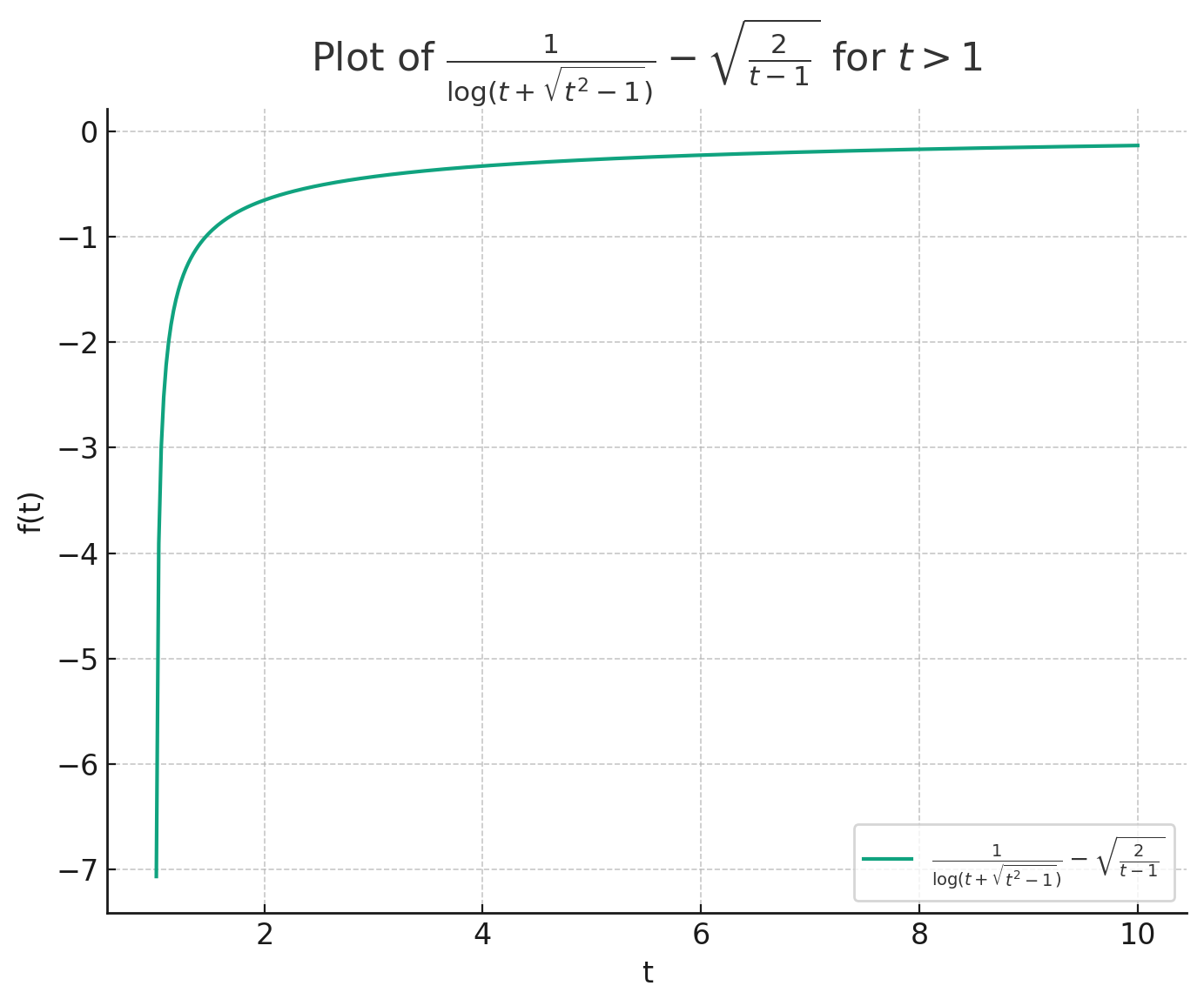
One can show, e.g., numerically that

$$\log \left(t+\sqrt{t^2-1}\right)^{-1} \le \sqrt{2/(t-1)} = \sqrt{\gamma_1^{-1}} = \sqrt{\frac{\lambda_2 -\lambda_n}{\lambda_1-\lambda_2}}$$

and thus

$$k \le 1+\sqrt{\frac{\lambda_2 -\lambda_n}{\lambda_1-\lambda_2}} \log \left( \frac{2\tan \angle\left(b, v_1\right)} {\sqrt{\varepsilon}}\right)$$

Note that

$$\tan \angle\left(b, v_1\right) =\frac{\sin \angle\left(b, v_1\right)}{\cos \angle\left(b, v_1\right)}=\frac{\sin \angle\left(b, v_1\right)}{\langle b, v_1\rangle}.$$

This completes the proof. □

Kuczyński’s Estimate

As the Lanczos method evolves the Krylov subspace, it is well known that convergence of both algorithms depends on the distribution of eigenvalues and on the angle $\angle(b, v_1)$; if orthogonal the method fails. Kuczyński ¹ started at an argument showing that $(a)$ for some fixed $b\in\mathbb{R}^n$, no Krylov-type algorithm can approximate $v_1 \in \mathcal{S}_1$ for all $A \in \mathcal{S}_n$; $(b)$ if a subspace of order $k$ (i.e., using $k$ iterations) is used, then there exists no algorithm to approximate $v_1$ in less than $n-1$ iterations. The central idea is to bypass the case when $b ~\perp~\mathcal{S}_1$ probabilistically. We use the original presentation. Consider

$$\left|\frac{\xi(A)-\lambda_1(A)}{\lambda_1(A)}\right| \leq \varepsilon$$

and by the nature of Lanczos method it equates to

$$\frac{\lambda_1(A) - \xi(A)}{\lambda_1(A)} \leq \varepsilon.$$

Denote $\lambda^{(k)}_1$ as the $k$-th approximate Ritz value. Two error metrics are in place for a distribution $\mu$,

$$e_{\mathrm{avg}}^{(k)} = \int_{\|b\|=1}\left|\frac{\lambda^{(k)}_1-\lambda_1(A)}{\lambda_1(A)}\right| \mu(db)$$

$$\mathbb{P}(\lambda^{(k)}_1, A, k, \varepsilon) = \mu\left\{b \in \mathbb{R}^n:\|b\|=1,\left|\frac{\xi(A, b, k)-\lambda_1(A)}{\lambda_1(A)}\right|>\varepsilon\right\}.$$

Expected error

We first consider the expected error.

We translate into convergence rates.

Proof: We show the second part. Let $\nu =\sqrt {\kappa_{\mathrm L}^{-1}}$, and let

$$2.589 \sqrt{n}\left(\frac{1-\nu}{1+\nu}\right)^{k-1} \le \varepsilon$$

$$\Rightarrow k \ge 1 + \log\left(\frac{2.589 \sqrt{n}}{\varepsilon}\right)/\log\left(\frac{1+\nu}{1-\nu}\right) = 1 + \log\left(\frac{2.589 \sqrt{n}}{\varepsilon}\right)/\log\left(1 + \frac{2\nu}{1-\nu}\right).$$

Since

$$\log\left(1 + 1/t\right) \ge \frac{1}{1/2 + t}$$

$$\Rightarrow \log\left(1 + \frac{2\nu}{1-\nu}\right) \ge \frac{1}{1/2 + \frac{1-\nu}{2\nu}} = 2\nu.$$

So safely state,

$$K = 1 + \left \lceil \frac{\sqrt{\kappa_{\mathrm L}}}{2}\log\left(\frac{2.589 \sqrt{n}}{\varepsilon}\right) \right \rceil.$$

□

Probabilistic bound

We now consider the probabilistic bound showing the error estimate holds with high probability $1-\delta$. This means $\mathbb{P}(\lambda^{(k)}_1, A, k, \varepsilon) \le \delta$.

Similar to the expected error, we can derive the convergence rates.

For completeness we provide the proof of the second part.

Proof: Let $\nu =\sqrt {\kappa_{\mathrm L}^{-1}}$, and let

$$1.648 \sqrt{\frac{n}{\varepsilon}}\left(\frac{1-\nu}{1+\nu}\right)^{k-1} \le \delta,$$

we have,

$$k \ge 1 + \log\left(\frac{1.648 \sqrt{n}}{\delta \sqrt{\varepsilon}}\right)/\log\left(\frac{1+\nu}{1-\nu}\right).$$

So safe to say,

$$K = 1+\left \lceil \frac{\sqrt{\kappa_{\mathrm L}}}{2}\log\left(\frac{1.648 n}{\delta \varepsilon}\right) \right \rceil$$

□

Taking the absolute error

If we consider the absolute error, then the above results can be translated therein by taking $\varepsilon = \epsilon/(\lambda_1-\lambda_n)$.

Consider a specific $A$, we can derive the following corollary.

Takeaways

An interesting recent paper discuss the behavior of Lanczos method in few iterations ³.

Acknowledgment

The author appreciates the discussion with Chang He that improves the presentation of this note.

References