How to inverse demand?

A few sufficient conditions and reading notes.

Introduction

Invertibility of demand is important for existence of an inverse demand function or (in an exchange economy) uniqueness of Walrasian equilibrium prices. In fact, it is also used in estimation of demand systems and testing of revealed preference, which would no longer limit demand shifters to prices.

In the context of general equilibrium theory ¹, Invertibility of demand refers to whether the mapping from prices to demands, $x(p)$, is one-to-one. If so, given a demand vector, we can recover the corresponding prices. Generally, existence of the market equilibrium is warranted by Brouwer’s fixed-point theorem, while uniqueness of it can be ensured by invertibility of demand. Granted, uniqueness may still be true without invertibility — the system may have a single solution even if it is degenerate somewhere.

Mathematically, if $\nabla x(p) = \frac{\partial x(p)}{\partial p}$ is the Jacobian, then local invertibility requires $\det(\nabla x) \neq 0.$

$P$-Matrix and Global Invertibility

One classical tool is to detect whether or not $x(p)$ is from the $P$-properties.

If the inequality is not strict, it is called $P_0$ matrix. By Gale–Nikaidô theorem ², $P$-functions are globally univalent (i.e., injective on $\mathbb{R}^n$). If $ -\nabla x(p)$ is a $P$-matrix for all $p$, the demand map is a $P$-function. Economically, gross substitutability often ensures a $P$-matrix, so equilibrium prices are unique.

We stop here and use the CES economy as a motivating example.

Starting Example: CES Demand

The CES utility with weights $c_j>0$ is $u(x) = \left(\sum_{i=1}^n c_j x_j^{\rho}\right)^{1/\rho}, \quad \sigma = \frac{1}{1 - \rho}~$ is the elasticity of demand. If there are some $c_j = 0$, simply consider the “active-set”: $B = \{j\in[n]\mid c_j > 0\}.$

Given prices $p$ and expenditure $m>0$, the Marshallian demand is
\[ x(p,w) = w P^{-1}\gamma, \quad \gamma_j(p)=\frac{c_j p_j^{1-\sigma}}{\sum_k c_kp_k^{1-\sigma}}, \quad \gamma \in \Delta_n. \]

The Fisher model: monetary endowment

In this case $w > 0$ is a fixed constant, then it is easy to see the Jacobian reads, \[ -\nabla x(p)=w P^{-1}\big[\ \sigma \Gamma +(1-\sigma)\,\gamma\gamma^\top\ \big] P^{-1}. \] I found this can actually be done easily by logarithmic homogeneity (see ³), a concept known for self-concordant barriers of self-scaled cones. For the Fisher case, $x(p)$ is always monotone. Actually, one could show,

\[| P ( x ( p + q )- x ( p )-\nabla x ( p )[ q ])| \leq \mathcal O\left(\frac{|P^{-1}q|^2}{2(1-|P^{-1}q|)}\right) \]

Arrow-Debreu trading setting

Now suppose income becomes $w(p)=b^\top p$. Hence, the Jacobian should be written as, \[ -\nabla x(p) = \underbrace{w P^{-1}\big[\ \sigma \Gamma +(1-\sigma)\,\gamma\gamma^\top\ \big] P^{-1}}_{A} - P^{-1}\gamma b^\top \] We have \[ (-\nabla x(p))p=w P^{-1}[\sigma \Gamma +(1-\sigma)\gamma\gamma^\top] P^{-1} - P^{-1}\gamma b^\top p-P^{-1}\gamma b^\top p=0 \]

Thus $\det(-\nabla x(p))=0$: the kernel is $\mathrm{span}\{p\}$. Work on the normalized price simplex (drop one price or restrict to the tangent space ${x:\,p^\top x=0}$). For any $I\subsetneq[n]$,

$$\det([-\nabla x(p)]_{I,I}) = \det(A_{I,I})(1-b_I^\top (A_{I,I})^{-1}(P^{-1}\gamma)_I).$$

A Sherman–Morrison calculation yields $(A_{I,I})^{-1}(P^{-1}\gamma)_I =\frac{1}{w}\,\frac{p_I}{\sigma+(1-\sigma)\,\gamma_I^\top\mathbf 1},$ this means

$$\det\big((-\nabla x(p))_{I,I}\big)>0\iff b_I^\top p_I<w\,[\,\sigma+(1-\sigma)\gamma_I^\top\mathbf 1\,].$$

Consequences

If $\sigma\ge1$, then $-\nabla x(p)$ is a $P_0$–matrix. For any proper $I \subsetneq [n]$, $\sigma+(1-\sigma)\gamma_I^\top\mathbf1\ge1$ and $b_I^\top p_I<w$, every proper principal minor is positive. The full determinant is $0$ (numéraire).

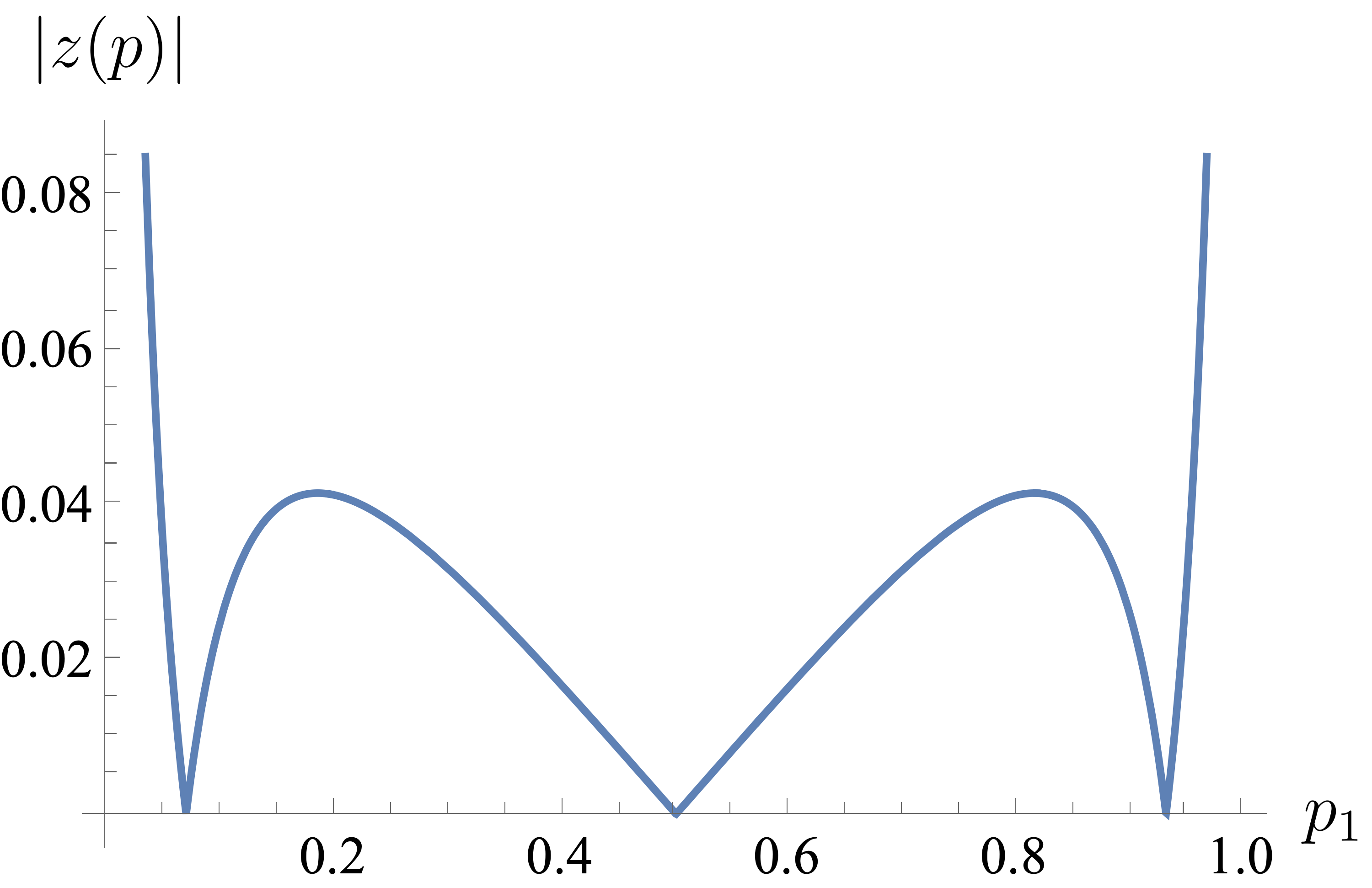
If $0<\sigma<1$: the inequality can fail for some $I$ (small $\gamma_I^\top\mathbf1$, large $b_I^\top p_I$), so the $P$–property on the simplex need not hold; multiplicity can occur. See the counter example below⁴.

Consider an Arrow–Debreu exchange market with two agents and two goods. Let both agents have $\rho_j = \rho = -3$ and $\sigma = \frac{1}{1 - \rho} = \frac{1}{4}.$ Their endowments and preferences are defined by $$b = \begin{bmatrix} 1 & 0 \\ 0 & 1 \end{bmatrix}, \quad c = \begin{bmatrix} a & 1 \\ 1 & a \end{bmatrix}, \quad a = \frac{2}{\Bigl(1 - 2\sigma\Bigr)^{\frac{1}{\sigma}}}.$$ Under the normalization $p_1 + p_2 = 1$, there are three disconnected equilibrium prices. (The symbol $z(p)$ is the excess, 0 indicates the equilibria prices.)

$P$-matrix (cont.)

Another well-known characterization is as follows ²:

(not finished…)

References